The Critical Chain/Buffer Management (CC/BM) approach uses project and feeding buffers to add safety time to the project baseline schedule and to guarantee the timely completion of the project with a high probability. Buffers are sized according to the properties of the path or chain feeding those buffers, such as the length of the path, its total variance or the number of activities it contains. This article describes the Root Squared Error Method (RSEM) to determine the size of the project and feeding buffers and is based on the predefined uncertainty of the activity durations of the chain merging in the buffer.
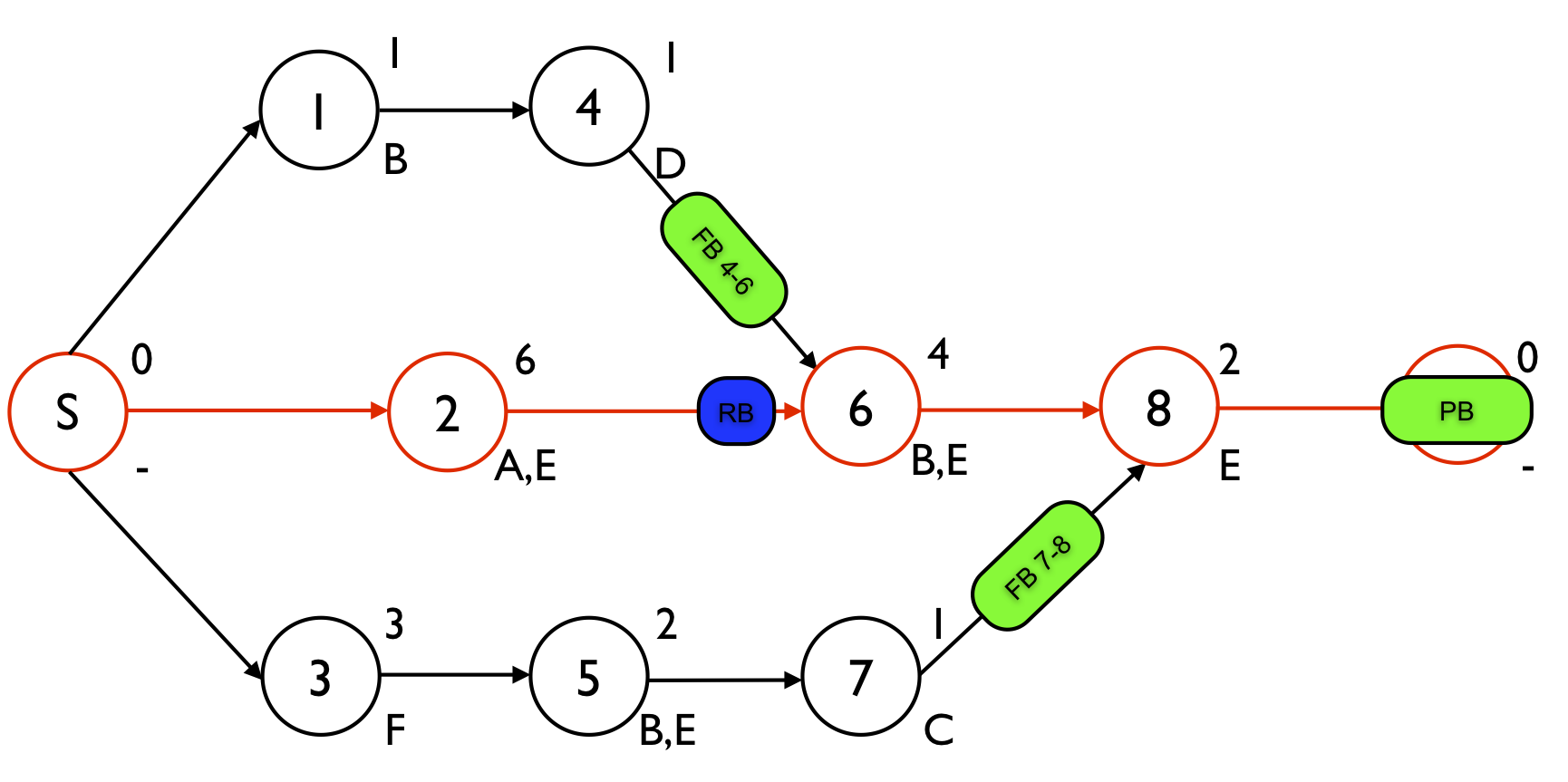
Figure 1 displays a project network with 8 activities. The numbers above each node are used to refer to the aggressive activity durations while the label below the node refers to a renewable resource that is required to perform the activity. The renewable resources A, B, C, D and F have an availability of one, while the renewable resource E availability is restricted to two units. The schedule contains three time buffers and one resource buffer. One project buffer is added to protect the critical chain S - 2 - 6 - 8 - E and two feeding buffers FB4-6 and FB7-8 are added to protect the feeding chains 1 - 4 and 3 - 5 - 7, respectively. The resource buffer RB is added to assure that resource B will be available on time to start with activity 6. More information on the determination of these buffers can be found at “
Critical Chain/Buffer Management: Adding buffers to a project schedule”.
?Figure 1. The project network with 2 feeding buffers, one resource and one project buffer
Table 1. Aggressive and safe activity durations
|
Activity |
1 |
2 |
3 |
4 |
5 |
6 |
7 |
8 |
|
Safe duration |
2 |
9 |
5 |
2 |
3 |
6 |
2 |
3 |
|
Aggressive duration |
1 |
6 |
3 |
1 |
2 |
4 |
1 |
2 |
Root Squared Error Method
Rather than using a simple rule-of-thumb to size project and feeding buffers, the sum of squares method accounts for known variation in activity durations. This method is often referred to as the sum of squares method since it takes the sum of the squared differences between the low risk duration and the aggressive duration into account.
?
buffer size
=
the square root of the sum of the squares of the difference between the low risk duration
and the aggressive duration for each activity along the chain leading to the buffer
In this method, the buffers are sized as the the square root of the sum of the squares of the difference between the low risk duration and the mean duration for each activity along the chain leading to the buffer, leading to the following values:
-
project buffer: sqrt((9 - 6)2 + (6 - 4)2 + (3 - 2)2) = sqrt(14) = 3.7
-
FB4-6: sqrt((2 - 1)2 + (2 - 1)2) = sqrt(2) = 1.4
-
FB7-8: sqrt((5 - 3)2 + (3 - 2)2 + (2 - 1)2) = sqrt(6) = 2.4
Rationale behind this method
It should be noted that the general underlying idea of this buffer method is that the size of these buffers is equal to two times the standard deviation of the path that merges into the buffer. Consequently, this buffer sizing rule depends on how the standard deviations of activities are defined.
In “
Critical Chain/Buffer Management: Sizing project and feeding buffers”, it has been assumed that the standard deviation of an activity is equal to 50% of the difference between the safe and aggressive durations. Assume that ∂
i is used to denote the difference between the safe and aggressive time estimate of activity i. The standard deviation of this activity is then equal to (∂
i / 2). As an example, ∂
2 is equal to (9 - 6) and the standard deviation of activity 2 is then equal to σ
2 = ( 9 - 6) / 2 = 1.5.
Assume that the chain consists of n activities 1, 2, ..., n. Since the buffer is sized as two times the path standard deviation, the buffer size is equal to:
2 * σpath = 2 * sqrt((∂1 / 2)2 + (∂2 / 2)2 + ... + (∂n / 2)2) = sqrt((∂1)2 + (∂2)2 + ... + (∂n)2)
which boils down to the buffer sizing rules used by the RSEM. As an example, the project buffer is sized as 2 * sqrt(1.52 + 12 + 0.52) = 3.7.
buffer size
=
two times the standard deviation of the
longest path in the chain
It should be noted that the advantage of the RSEM is that it takes known variation in the activity duration into account, and it can therefore be considered as a more elaborated technique than the simple 50% rule (see “
Sizing CC/BM buffers: The cut and paste method”). However, this technique has also been criticized in literature since it may lead to undersized buffers when chains are relatively long due to the underestimation of activity variation. To that purpose, a variant of the method, known as the “bias plus sum of the squares
” method has been proposed which combines the 50% rule and the RSEM. More details are outside the scope of this article. An overview of other buffer sizing methods is available at “Critical Chain/Buffer Management: Sizing project and feeding buffers”.