The Critical Chain/Buffer Management (CC/BM) approach uses project and feeding buffers to add safety time to the project baseline schedule and to guarantee the timely completion of the project with a high probability. Buffers are sized according to the properties of the path or chain feeding those buffers, such as the length of the path, its total variance or the number of activities it contains. This article describes the adaptive procedure with density method, in which the size of the buffers is based on the structure of the subnetwork that feeds into buffer.
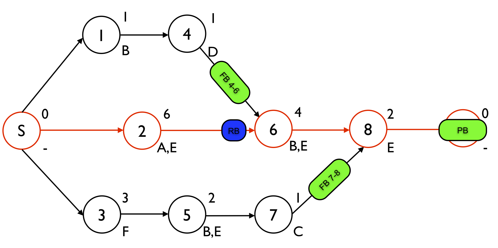
Figure 1 displays a project network with 8 activities. The numbers above each node are used to refer to the aggressive activity durations while the label below the node refers to a renewable resource that is required to perform the activity. The renewable resources A, B, C, D and F have an availability of one, while the renewable resource E availability is restricted to two units. The schedule contains three time buffers and one resource buffer. One project buffer is added to protect the critical chain S - 2 - 6 - 8 - E and two feeding buffers FB4-6 and FB7-8 are added to protect the feeding chains 1 - 4 and 3 - 5 - 7, respectively. The resource buffer RB is added to assure that resource B will be available on time to start with activity 6. More information on the determination of these buffers can be found at “Critical Chain/Buffer Management: Adding buffers to a project schedule”.
?Figure 1. The project network with 2 feeding buffers, one resource and one project buffer
The adaptive procedure with density
The rationale behind buffer sizing methods based on network density is that subnetworks with an increasing number of precedence relations for a given number of activities have a high chance to cause delays. To that purpose, the so-called adaptive procedure with density (APD) has been proposed, which takes the density of the subnetworks that feed into the buffer into account. Buffers are sized according to these subnetwork density values to assure that a higher number of precedence relations leads to a bigger buffer size to increase their power to absorb potential delays.
The buffer is sized as the standard deviation of the path leading to the buffer scaled by a factor which is calculated by taking the density of the subnetwork merging into the buffer into account, as follows:
Buffer size = K x σpath
with
K: The scaling factor based on the subnetwork density
σpath: The standard deviation of the longest path feeding the buffer.
buffer size
=
standard deviation of the path leading to the buffer scaled by a factor
which is calculated by taking the resource density into account.
In the following sections, the calculations of the path standard deviations, the density of the subnetworks and the scale parameter K are illustrated on the example network of figure 1.
Standard deviation
The standard deviation of the longest path can be calculated in various ways. In this article, it is assumed that the standard deviations of the activities are equal to 50% of the difference between the safe and aggressive durations (see table 1). The standard deviation σpath of a path is then equal to the square root of the sum of the variances of the activities on that path, as follows:
-
Critical chain 2 - 6 - 8: sqrt(1.52 + 12 + 0.52) = 1.87
-
Feeding chain 1 - 4: sqrt(0.52 + 0.52) = 0.71
-
Feeding chain 3 - 5 - 7: sqrt(12 + 0.52 + 0.52) = 1.22
Table 1. Aggressive and safe activity durations
|
Activity |
1 |
2 |
3 |
4 |
5 |
6 |
7 |
8 |
|
Safe duration |
2 |
9 |
5 |
2 |
3 |
6 |
2 |
3 |
|
Aggressive duration |
1 |
6 |
3 |
1 |
2 |
4 |
1 |
2 |
Network density
The network density of a subnetwork merging into the buffer is a measure of how dense the network is in terms of the number of activities and precedence relations between these activities. The network density used in the adaptive procedure with density is equal to the number of precedence relations divided by the number of activities in the subnetwork, but obviously many alternatives could have been used. This density value is known as the coefficient of network complexity (CNC).
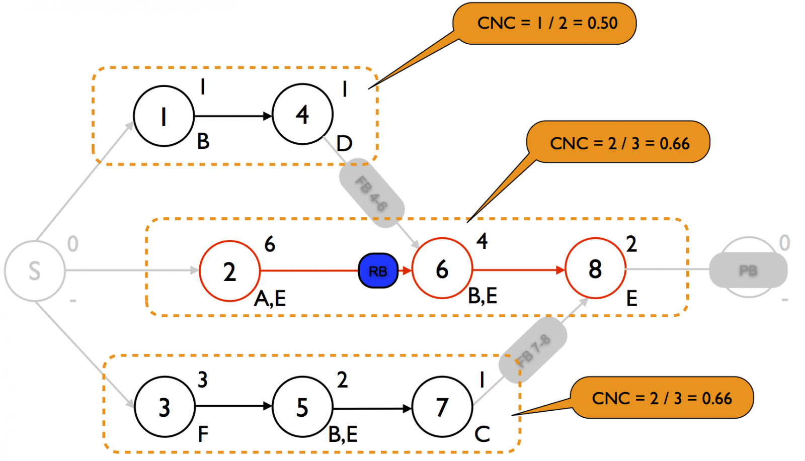
?Figure 2. Three subnetworks merging into a buffer with their CNC value
Figure 2 shows the three subnetworks for the three time buffers with their corresponding density values. Since the first node (S) and the last node (E) are dummy nodes with a zero duration and no resource demand, the precedence relations connected to these nodes are excluded from the calculations.
It should be noted that the three subnetworks in figure 2 are all single paths. In more complex project networks, these subnetworks can consist of networks with serial and parallel activities. In this case, the coefficient of network complexity used to measure the subnetwork density should take the complete network into account, and not only the longest path. The calculation of the path standard deviation, on the other hand, only takes the longest path of the subnetwork into account.
Scale parameter K
The network density is then used to calculate the scale factor K that is equal to
K = 1 + network density
The buffer sizes based on the adaptive procedure with density are then equal to:
-
Project buffer: 1.66 * 1.87 = 3.10
-
FB4-6: 1.50 * 0.71 = 1.07
-
FB7-8: 1.66 * 1.22 = 2.03
The rationale behind this buffer sizing method that a higher number of precedence relations for the same number of activities is possibly more sensitive to delays makes sense. When the coefficient of network complexity increases, it is indeed more likely that delays will occur more often and therefore larger buffers should be added that are able to absorb these delays. An overview of other buffer sizing methods is available at “
Critical Chain/Buffer Management: Sizing project and feeding buffers”.