Critical Chain/Buffer Management: Sizing project and feeding buffers

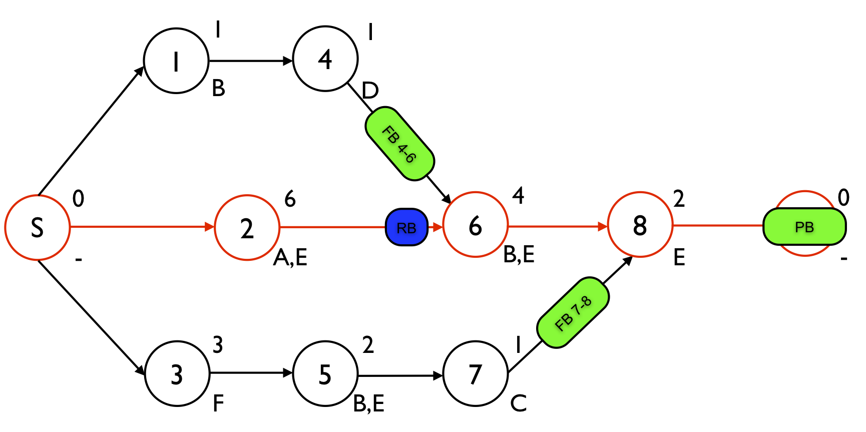
The Critical Chain/Buffer Management (CC/BM) approach uses project and feeding buffers to add safety time to the project baseline schedule and to guarantee the timely completion of the project with a high probability. Buffers are sized according to the properties of the path or chain feeding those buffers, such as the length of the path, its total variance, its average resource use or the number of activities it contains. In this article, a non-exhaustive overview of buffer sizing methods is given. Moreover, an example project is given in figure 1 which is based on other CC/BM articles and which will be used to illustrate the different buffer sizing methods in detail in other articles.

Figure 1 displays a project network with 8 activities. The numbers above each node are used to refer to the aggressive activity durations while the label below the node refers to a renewable resource that is required to perform the activity. The renewable resources A, B, C, D and F have an availability of one, while the renewable resource E availability is restricted to two units. The schedule contains three time buffers and one resource buffer. One project buffer is added to protect the critical chain S - 2 - 6 - 8 - E and two feeding buffers FB4-6 and FB7-8 are added to protect the feeding chains 1 - 4 and 3 - 5 - 7, respectively. The resource buffer RB is added to assure that resource B will be available on time to start with activity 6. More information on the determination of these buffers can be found at “Critical Chain/Buffer Management: Adding buffers to a project schedule”.
 
?Figure 1. The project network with 2 feeding buffers, one resource and one project buffer 
 
Table 1 is an overview table that displays the safe and aggressive durations of all project activities based on the example given in “Critical Chain/Buffer Management: (Dis-)advantages of scheduling projects as-late-as-possible”. The difference between the safe and aggressive time estimates is also indicated in the column with label ‘delta duration’. The use of aggressive time estimates is discussed in “Aggressive activity time estimates: protecting against activity delays”.
 
Table 1. Summary of project data
Activity Safe duration Aggressive duration Delta duration Standard deviation
1 2 1 1 0.5
2 9 6 3 1.5
3 5 3 2 1.0
4 2 1 1 0.5
5 3 2 1 0.5
6 6 4 2 1.0
7 2 1 1 0.5
8 3 2 1 0.5
 
In table 1, the standard deviations of the activities are assumed to be 50% of the difference between the safe and aggressive durations. Although this has been suggested in literature, obviously other values can be set based on more detailed risk information and known or estimated distributions of activity durations. For more information on using distributions on activity parameters, see “Project risk: Statistical distributions or single point estimates?”. Alternatively, the standard deviation can also be based on three point estimates as is the case in the PERT method (see “The Program Evaluation and Review Technique (PERT): Incorporating activity time variability in a project schedule”).
 
Given the assumed values for the activity standard deviations, the standard deviation σpath of a path is then equal to the square root of the sum of the variances of the activities on that path. In this case, it is assumed that the activity finishing times are independent (an assumption which also has been taken by the PERT technique). As an example, the standard deviation of the critical chain is equal to: 
  • Critical chain 2 - 6 - 8: sqrt(1.52 + 12 + 0.52) = 1.87
  • Feeding chain 1 - 4: sqrt(0.52 + 0.52) = 0.71
  • Feeding chain 3 - 5 - 7: sqrt(12 + 0.52 + 0.52) = 1.22
In table 2, an overview is given of five methods to determine the size of the buffers. Each method is briefly described and a link to a more detailed example is given. In these referenced articles, the network of figure 1 and the values of table 1 will be used as inputs.
 
Table 2. An overview of five buffer sizing methods used in Critical Chain/Buffer Management
Buffer size method Description Reference
Cut and paste method Buffer sizes are based on the duration of the chain feeding the buffer Sizing CC/BM buffers: The cut and paste method
Root Squared Error Method Buffer sizes are based on risk in the activity durations Sizing CC/BM buffers: The root squared error method
Adaptive procedure with density (APD) Buffer sizes are based on the structure of the partial network to which the chain belongs Sizing CC/BM buffers: The adaptive procedure with density
Adaptive procedure with resource tightness (APRT) Buffer sizes are based on the average resource use of the resources used by the activities on the longest path of the chain Sizing CC/BM buffers: The adaptive procedure with resource tightness

© OR-AS. PM Knowledge Center is made by OR-AS bvba Contact us at info@or-as.beVisit us at www.or-as.beFollow us at @ORASTalks