Earned Value Management: Reliable time performance measurement

Submitted by Mario Vanhoucke on Mon, 12/12/2011 - 17:26

Controlling a project is key to the success or failure of the project. Earned Value Management (EVM) is a well-known technique to control the time and cost performance of a project and to predict the final project duration and cost. It is an easy tool to generate early warning signals to timely detect project problems or to exploit project opportunities. In “Earned Value Management: The three key metrics”, it has been discussed that EVM relies on three key input metrics, known as the planned value (PV), the actual cost (AC) and the earned value (EV). In “Measuring Time: Earned value or earned schedule?”, it has been shown that a fourth method, known as Earned Schedule (ES), works better for measuring the time progress of a project.

In this article, the schedule performance index SPI is criticized for its unreliable behavior towards the end of a project and an alternative schedule performance index SPI(t) is presented. Example calculations will be used to illustrate this issue, based on the baseline schedule and fictitious project progress of a project that ends 2 weeks later than planned, as shown in figure 1. The baseline schedule displays the cumulative planned values for each activity and the real-life execution shows the cumulative actual costs for each activity.

An overview of the EVM metrics is given in “Earned Value Management: An overview” and the formulas are summarized in “Earned Value Management: The EVM formulary”.

Figure 1: An example project baseline schedule (top) and real-life progress (bottom) with 2 weeks delay

Project performance

A project’s time performance is measured by the schedule variance SV or the schedule performance index SPI, as discussed in “Earned Value Management: Measuring a project’s performance”. However, the Earned Schedule technique allows to measure alternative versions of the schedule performance index and variance, as follows:

Schedule Variance (SV(t)): Shows the variance in time (ES - AT) expressed in time units
- > 0: project ahead of schedule
- = 0: project on time
- < 0: project delay
Schedule Performance Index (SPI(t)): Shows the performance of time (ES / AT) in a unitless dimension
- > 100%: project ahead of schedule
- = 100%: project on time
- < 100%: project delay

with AT = the current Actual Time (e.g. week 7 in figure 2).

Figure 2 shows the schedule variances SV and SV(t) on the example project of figure 1 at week 7. While SV measures the schedule performance not in units of time, but rather in costs, the SV(t), instead, measures the project progress in a time dimension. However, the earned schedule technique, and its alternative performance measures, have another advantage which is more important than the simple expression in time units instead of costs: it solves the unreliable behavior of the traditional SPI metric.

Figure 2: Real life execution (project progress at week 7)

Table 1: The EVM data for the example project of figure 1

	W1	W2	W3	W4	W5	W6	W7	W8	W9	W10	W11
AT	1	2	3	4	5	6	7	8	9	10	11
PV	5.00	10.00	25.00	55.00	85.00	120.00	130.00	140.00	150.00	150.00	150.00
AC	10.00	20.00	30.00	75.00	120.00	155.00	170.00	195.00	200.00	205.00	210.00
EV	3.33	6.67	10.00	22.50	70.00	82.50	90.00	120.00	130.00	140.00	150.00
ES	0.67	1.33	2.00	2.83	4.50	4.92	5.14	6.00	7.00	8.00	9.00
SV	-1.67	-3.33	-15.00	-32.50	-15.00	-37.50	-40.00	-20.00	-20.00	-10.00	0.00
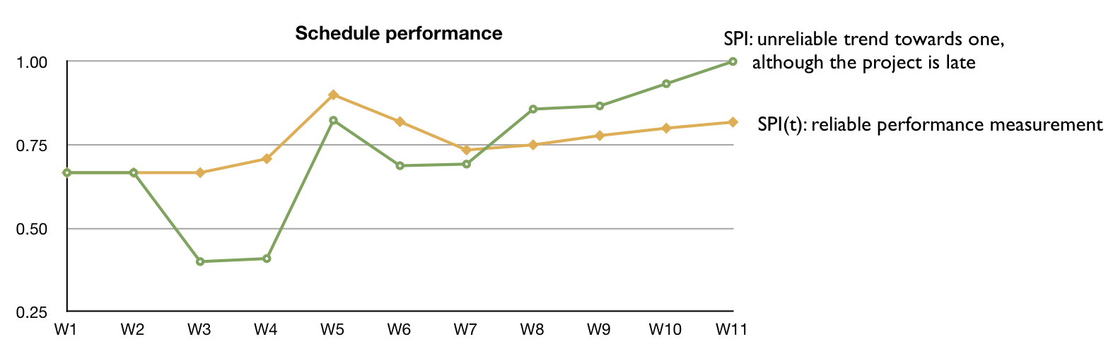
SPI	0.67	0.67	0.40	0.41	0.82	0.69	0.69	0.86	0.87	0.93	1.00
SV(t)	-0.33	-0.67	-1.00	-1.17	-0.50	-1.08	-1.86	-2.00	-2.00	-2.00	-2.00
SPI(t)	0.67	0.67	0.67	0.71	0.90	0.82	0.73	0.75	0.78	0.80	0.82

Table 1 shows the EVM metrics along the project duration (11 weeks) of figure 1. The table shows the following observations at the end (week 11) of the project:

PV varies between € 0 (at the start of the project) and the budget at completion (BAC) at the end of the project.
EV varies between € 0 (at the start of the project) and the budget at completion (BAC) at the end of the project.
ES varies between 0 time units (at the start of the project) and the baseline Planned Duration (PD) at the end of the project.

Hence, at the end of the project, EV = PV and ES = PD. Based on this fact, the performance indicators show the following behavior at the project end:

SV = EV - PV = BAC - BAC = 0 (when project is on time or late)
SPI = EV / PV = BAC / BAC = 1 (when project is on time or late)
SV(t) = ES - AT = PD - AT
- > 0, if AT < ES (project is early)
- = 0, if AT = ES (project is on time)
- < 0, if AT > ES (project is late)
SPI(t) = ES / AT = PD / AT
- > 1, if AT < ES (project is early)
- = 1, if AT = ES (project is on time)
- < 1, if AT > ES (project is late)

Consequently, since the Earned Value metric EV is always equal to the Planned Value metric PV at the end of the project, the SPI always ends at 100%, regardless of the real project state (on time or late). This unreliable trend of the SPI towards 1 at the end of the project has been the topic of many discussions and research projects, which is solved when using the alternative SV(t) and SPI(t) performance measures. Figure 3 displays the SPI and SPI(t) for the example project.

?Figure 3: SPI versus SPI(t)

PM Knowledge Center

Earned Value Management: Reliable time performance measurement